Let me introduce you to time-series factor momentum, a strategy that attempts to harness the auto-correlation in factor returns (see Gupta & Kelly (2019) for a comprehensive study). Factor returns are frequently significantly auto-correlated, which investors can utilize to time factor returns. For example, consider the value factor in which we buy low book-to-market stocks (value stocks) and sell high book-to market stocks (growth stocks). The value factor exhibits relatively high auto-correlation and yields relatively high time-series factor momentum returns. The time-series factor momentum strategy buys the value factor (long position) if the prior month’s return was positive and sells the value factor (short position) if the prior month’s value factor return was negative or zero. The return to the strategy of an arbitrary factor i is shown in the equation below.
![]()
![]()
![]()
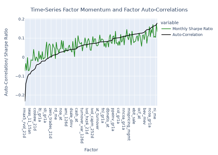
Compared to the mere holding of the factor, this strategy earns higher returns. Since I do not attempt to match different time-series factor momentum strategies, I waive volatility scaling throughout this article. I use the data of Jensen, Kelly & Pedersen (2021), which is kindly provided by Professor Bryan Kelly on his homepage. In the figure below, we find factor auto-correlation being highly correlated with the performance of time-series factor momentum strategies.

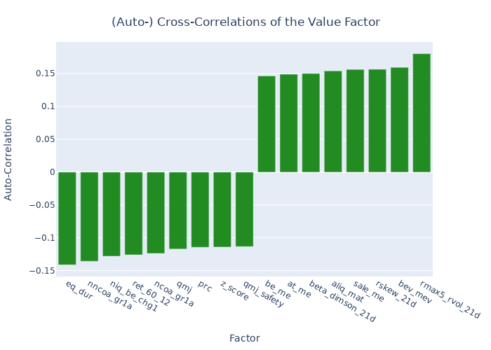
Next, I want to show you that the already promising results of time-series momentum can be further boosted by a phenomenon I call “cross-correlation time-series factor momentum” (CC-TS-FMom). Instead of observing prior realizations of one factor, I calculate auto-cross-correlations between the whole set of 153 factors. Other factors that tend to drive the factor of interest show higher correlations with future observations of the factor than the factor itself. The figure below shows auto-cross-correlations of the value factor. The value factor itself, despite being one of the highly auto-correlated factors, is overarched in terms of auto-cross-correlation by several other factors. Additionally, we find factors (e.g. long-term reversal/ ret_60_12) to negatively drive future value factor returns.

Similar to the time-series momentum strategy, the cross-correlation time-series factor momentum strategy either holds pure long (w=1) or pure short positions (w=-1) depending on prior month returns. Because we want to investigate multiple factors’ impact on future returns, we need to implement a suitable measure accounting for all factors. Instead of using the prior month’s own-factor return, we calculate the median of normalized driving factors returns. Driving factors are defined as the top and low decile auto-cross-correlation factors. The normalization swaps the sign for the negatively cross-correlated factors. The strategy is shown in the equation below.
![]()
![]()
![]()
![]()
![]()
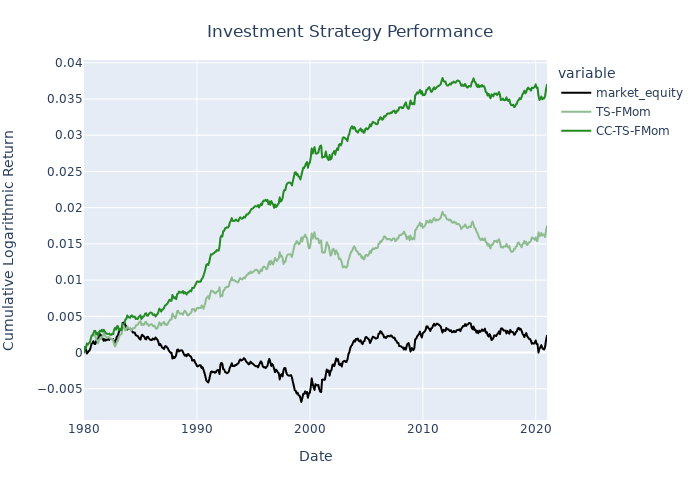
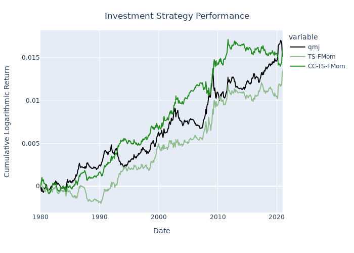
The strategy buys a factor i in t+1 when the median of the sign adjusted returns r of the driving factors d is positive in t. The strategy sells the factor i in t+1, when the median is negative respectively. The driving factors d are the factors in the highest and lowest decile of cross-correlation R with the factor i. This simple strategy is able to beat time-series factor momentum in the majority of factors. The figures below exhibit the investment performance of pure factor portfolios, time-series factor momentum portfolios and cross-correlation time-series factor momentum portfolios for three different popular investment factors: Value, Size, and Quality.


