Recently, I presented two new concepts related to risk factor cross-correlations. Namely, I showed you cross-correlation time-series factor momentum and I used deep neural networks to predict the returns of the value factor. Today I want to expand the application of deep learning towards a custom-designed loss function. Instead of using standard loss functions like mean squared error, a quantitative investor might consider implementing optimizing on a function that is more closely related to the investment process. As we found in the last post, even relatively high out-of-sample coefficients of determination do not guarantee superior investment performance. In this post, I will introduce you to deep position sizing using neural networks.
In their standard setup, supervised deep learning attempts to model the mapping of a target feature y to a feature space X by minimizing a mean squared error loss function. This supervised learning setup comes with a severe limitation, as it forces the investor to process noisy return predictions into investment decisions, a two-step approach. Instead, we can directly model the investment position p̂ as a function of the same features X, which we used to predict the stock returns. This procedure shrinks the two-step approach into one single step. Consider the loss function L:
![\[L(r, \hat{p})=-\frac{1}{T} \sum_{t=1}^T ( r_{t} \times \hat{p}_{t} - \hat{p}_{t} ^ \lambda) \]](https://merlinbartel.com/wp-content/ql-cache/quicklatex.com-e110265a996ca29e2e72a266581c16ed_l3.png "Rendered by QuickLaTeX.com")
![\[ with \]](https://merlinbartel.com/wp-content/ql-cache/quicklatex.com-c3215180851bd46d97ce850786fa9ed2_l3.png "Rendered by QuickLaTeX.com")
![\[ \hat{p}_{t}=f(r_{d,t-1},r_{d+1,t-1}...,r_{D,t-1}) \]](https://merlinbartel.com/wp-content/ql-cache/quicklatex.com-c54e83838b9f7717a1513aa45dda0fc4_l3.png "Rendered by QuickLaTeX.com")
The minimization of the loss function L is substantially different from minimizing losses like mean squared error. The model finds the optimal position size p at time t in a way to maximize our investment performance. After optimization, we normalize the absoulte sum of positions to equal the total amount of out-of-sample months. This procedure is necessary to assure comparability to time-series factor momentum, which holds the same abolute amount. The penalty parameter λ regularizes the maximum and minimum weights and forces both to stay in the range between -2 and +2. The optimal investment position p is modeled as a function of all prior month driving factor returns rD. A factor is considered as a driving factor d if it belongs to the highest or lowest decile of cross-correlation coefficients Ri,d.
One of the major disadvantages of mean squared error is its equal handling of positive and negative errors. For an investor anyhow, distinguishing negative and positive returns is of primary importance. Deep time-series factor momentum covers this importance and achieves a higher hit ratio (which is the proportion of times that the prediction guesses the sign of the return correctly), than both simple time-series factor momentum and predicted time-series factor momentum. The figure below plots the hit ratios of the three strategies for the US size factor.

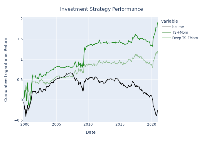
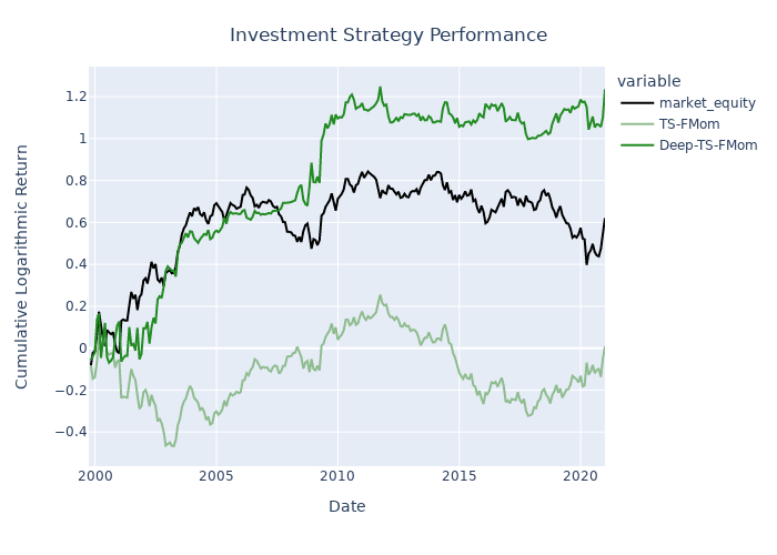
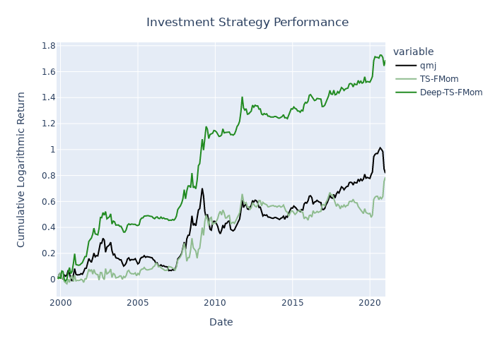
The deep time-series factor momentum strategy beats both the simple holding of the factor at hand and a simple time-series factor momentum strategy for most of the 153 US factors in the dataset of Jensen, Kelly & Pedersen (2021), which is kindly provided by Professor Bryan Kelly on his homepage. The figures below exhibit the investment performance of pure factor portfolios, time-series factor momentum portfolios and deep time-series factor momentum portfolios for four different popular investment factors: Value, Size, and Quality.